Tutorial

This tutorial is intended as a quick-start guide to show you, how you can average and reconstruct your hologram series. It assumes you are familiar with the general hologram reconstruction routine. A more thorough description of the general reconstruction can be found in textbooks. For instance, the chapter on electron holography in “Carter and Williams (Eds.), Transmission Electron Microscopy, Diffraction, Imaging, and Spectrometry, Springer” (the companion volume) covers these aspects.

Prerequisites

Obviously, holoaverage must be properly installed on your local computer (see Installation).

This tutorial shows how the required parameters for the reconstruction and averaging of a hologram series can be obtained in Digital Micrograph 2.30 by Gatan Inc. (also known as Gatan Microscopy Suite). Other microscopy software provides similiar capabilities to evaluate your data and can be used accordingly.

Furthermore a text editor is needed for writing and editing the parameter files provided to holoaverage. You can use your favorite text editor for this (this is not the same as word processing software), just make sure you save your files in “UTF-8” encoding (e.g. when you use Windows’ notepad for this, select “UTF-8” in the encoding field in the save dialog; see the article on Wikipedia, if you want to learn more about encoding).

Data files

This tutorial uses a high-resolution holographic focal series of a GaN as example. This focal series is available as zip-archive from the DOI 10.14279/depositonce-6674.

Unzip the contents into a directory. You will see that actually two hologram series are contained, one with the GaN crystal in one partial wave. These are the files a1_001.dm3, a1_002.dm3, a1_003.dm3, … .

The other hologram series was obtained without an object in the beam and is used for normalization (flat-field correction). These are the files empty_001.dm3, empty_002.dm3, … .

Overview

The main input to the program is a series of object holograms. Off-axis holograms interfere two regions of the specimen. In object holograms one of these regions is the area of interest, the other is the reference region (typically a vacuum area). This is in contrast to empty holograms, where typically both regions only contain vacuum.

The program performs roughly these steps:

1. Reconstruction of empty hologram series
2. Alignment and averaging of the reconstructed empty holograms
3. Raw alignment of the object hologram series
4. Reconstruction of the object hologram series
5. Flat field correction of the reconstructed object holograms by the averaged empty hologram
6. Alignment and averaging of the reconstructed object holograms

The alignment and averaging steps of both hologram series are done iteratively. Details on the program flow are given in the section Overview. Details on the whole alignment procedure can be found in

T. Niermann and M. Lehmann

Averaging scheme for atomic resolution off-axis electron holograms

Micron 63 (2014) 28-34

doi: 10.1016/j.micron.2014.01.008

The empty hologram series is only aligned for a global amplitude and phase factor (effects of filament instability). Four iterations of the averaging loop are performed. If enabled (see adjust_tilt) it is also aligned for the drift of biprism voltage.

The object hologram series is additionally aligned for specimen drift (which can be disabled by adjust_shift), and focal drift (if enabled by adjust_defocus). Seven iterations of the averaging loop are performed, the focal drift alignment is only done in the last three iterations.

Despite the name of the above mentioned paper, the averaging scheme also works for other kind of holographic reconstructions, e.g. medium resolution holography, or geometric phase analysis.

Creating the parameter file

Create a text file in the directory, where you unzipped your data files. The text file will contain the parameters used for the reconstruction and averaging. Copy the following text into this file and save it under the name holoaverage-a1.json. You can choose the name of the parameter file freely, however we will assume you called it holoaverage-a1.json in the following. We will discuss the meaning of the most important parameters in the following. A thorough reference for all parameters can be found in the Section Parameters of the documentation. Lines beginning with double slashes (i.e. //) are comments and are ignored by the program.

{
    // Path of hologram files (using printf format, integer argument). Required.
    "object_names" : "a1_%03d.dm3",

    // Index of first hologram.
    "object_first" : 1,

    // Index of last hologram. Required.
    "object_last" : 20,

    // Same (name, first index, last index) for "empty" holograms.
    "empty_names" : "empty_%03d.dm3",
    "empty_first" : 1,
    "empty_last" : 20,

    // Sampling (nm/px) of object holograms.
    // Defaults to value in data files.
    "sampling" : 0.00519824,

    // Voltage in kV. Default to value recorded in data files.
    "voltage": 300,

    // Defocus of first hologram (i.e. object_first) in nm. Defaults to 0.
    "defocus_first" : 20.0,

    // Defocus step size in nm. Defaults to 0.
    "defocus_step" : -2.0,

    // Size (in px) used for reconstruction of "empty" holograms. Required.
    "empty_size" : 512,

    // Size (in px) used for reconstruction of "object" holograms Required.
    "object_size" : 384,

    // X, Y Position of sideband in FFT pixels (origin is in center). Required.
    "sideband_pos" : [1136, 1304],

    // Reconstruction region in pixels (L, T, R, B). Defaults to full region.
    "roi" : [128, 128, 1920, 1920],

    // Region for raw alignment in pixels (L, T, R, B). Defaults to roi.
    //"align_roi" : [256, 256, 1536, 1536],

    // Disable raw alignment. Raw alignment is enabled by default.
    //"enable_raw_alignment" : false,

    // Output file name (will be HDF5 file). Required.
    "output_name" : "a1.hdf5",

    // Mask type (see FilterFunction for details). Defaults to "EDGE"
    // "filter_func" : "EDGE",
    "filter_func" : ["BUTTERWORTH", 14],

    // cut off frequency in 1/nm (q_max). Required.
    "cut_off" : 14.5,

    // Parameterization for MTF
    "mtf" : [["CONSTANT", -2.25536738e-02],
             ["LORENTZIAN", 1.02543658e-05, 1.15367655e-04],
             ["LORENTZIAN", 2.49224357e-02, 5.35262063e-02],
             ["GAUSSIAN", 4.60461599e-01, 4.36842560e+02]],

    // Correct phase by empty phase only (true), or full complex reconstruction (false).
    // Defaults to false.
    "only_phase": false,

    // Optimize defocus. Default: false
    "adjust_defocus" : true,

    // Optimize shift. Default: true
    "adjust_shift" : true
}

Setting the input files

At first the file names for the input files must be provided. Here we have two series, the series of the object holograms, i.e. a1_XXX.dm3, and the series of the empty holograms, i.e. empty_XXX.dm3. The first parameter object_names describes, how the object holograms are named:

"object_names" : "a1_%03d.dm3",

Our holograms have filenames starting with a1_, followed by a three digit number, and have the extension .dm3. The %03d in the filename describes, how the number is encoded in the filename (here 3 digits, zero padded). If our filenames, for instance, would be called a1.1.dm3, a1.2.dm3, a1.3.dm3 …, we would set the object_names parameter to a1.%d.dm3, where the %d would mean just a decimal number with as many digits as needed. If you interested, how to encode other numbers, look at the old-style formating rules of python.

The next two parameters give the range of numbers contained within the series:

"object_first" : 1,
"object_last" : 20,

Here, the series starts at index 1 and ends at index 20 (inclusive).

The next parameters describe, how the empty hologram series is named. These parameters follow the same conventions as the parameters described above.

"empty_names" : "empty_%03d.dm3",
"empty_first" : 1,
"empty_last" : 20,

The microscope parameters

The example holograms provided here are not correctly calibrated. The holograms were recorded using a non standard setup of the microscope, which is not correctly identified by the recording software. For this reason it is needed to provide the correct calibration to the holoaverage program. The correct calibration is specified by the parameter sampling and gives the size of one pixel in nanometers. When the sampling parameter is present, it overrides any calibrations from the image files. If the parameter is not present in the parameter file, the calibrations are taken from the image files.

Here, the material recorded in the holograms is well known, thus the reflections in the Fourier transforms of the holograms were used for calibration. The following setting makes the correct calibration known to the program

"sampling" : 0.00519824,

If you are used to Digital Micrograph, you can find the sampling of an image under “Calibrations” in the “ImageDisplay…” dialog available, when you right-click an image.

The holoaverage program also has to know the acceleration voltage of the microscope. In this case, it could also read it from the image files itself (i.e. omitting this parameter). Nevertheless, we provide it here in kilovolts:

"voltage": 300,

In this case the object series is a holographic focal series, which means the defocus is changing from hologram to hologram. The holoaverage program will propagate all holograms to the Gaussian focus. The parameter defocus_first gives the defocus of the first hologram (given by object_first) in nanometers (overfocus is positive). The parameter defocus_step gives the increment / decrement of the defocus between two consecutive images of the series. Here the first hologram is taken with a defocus of (estimated) 20 nanometers, the second with a defocus of (estimated) 18 nanometers. So the defocus is decremented by 2 nanometers, between two consecutive acquisitions:

"defocus_first": 20,
"defocus_step": -2,

Please note, that the reconstructions are propagated to the Gaussian focus (defocus 0 nm), as given by the defocus parameters above. When wrong parameters are provided, this the target focus is not the Gaussian focus. The resulting holograms can nevertheless propagated to a different focus afterwards. If no defocus parameters are provided, no propagation is performed, and the program averages all reconstructed holograms as they are.

The final parameter describing the microscope, is the modulation transfer function (MTF) of the camera. This MTF must be provided to the holoaverage program. As it is practice in most labs to describe the MTF as a parameterization of some simple functions, this parameterization can be directly provided to the program. This description is documented in Section Modulation Transfer Function. For this tutorial we simply pass the provided MTF to the program. If you don’t know the MTF of your detector, you can omit this parameter in the parameter file. Obviously no MTF correction is performed in this case.

"mtf" : [["CONSTANT", -2.25536738e-02],
         ["LORENTZIAN", 1.02543658e-05, 1.15367655e-04],
         ["LORENTZIAN", 2.49224357e-02, 5.35262063e-02],
         ["GAUSSIAN", 4.60461599e-01, 4.36842560e+02]],

Reconstruction parameters

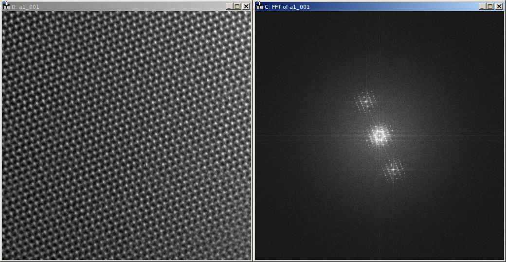
The holoaverage program has to know the carrier frequency of your hologram. This carrier frequency is most conveniently identified as the position of the sideband in one of the Fourier transformed empty holograms. In Digital Micrograph you can use the point ROI tool. This is the central tool button in the ROI toolbar looking like a cross-hair (if this toolbar is not visible, enable it in the “Toolbars” tab of the “Window/Customize…” dialog):

Selecting the center of the desired sideband allows to read out the coordinates of the sideband. Which of the two sidebands is the correct one, depends on the convention you use for your phase and on which side of the biprism your object was located. We use the convention that the phase shift increases with increasing specimen thickness. In this case, the correct sideband is the one, which is located on the side of the biprism filament, where the reference wave passed. In this GaN example, the biprism filament was oriented in 8 to 2 o’clock orientation. The object partial wave passed the top side of the filament, the reference partial wave the bottom side. Thus we select the lower side band here, located in the 5 o’clock position.

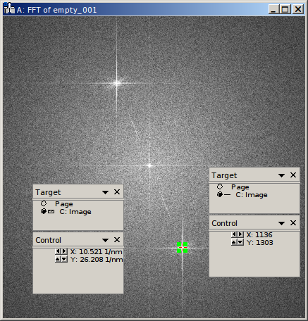
With the marker positioned on the sideband, the coordinates of the sideband can be read in the “Control” panel (if not visible, enable it in the “Window/Floating Window” drop down menu). The “Control” panel actually has two modes, either showing the position in calibrated units (see left part of the above figure) or as pixel position (right part of the above figure). You can toggle the mode by clicking on the little scalebar in the “Target” panel (in the figure above directly left to “C:Image”). For the parameter file we need this position in pixels. This position is given by the sideband_pos parameter as X and Y coordinates:

"sideband_pos" : [1136, 1304],

When the sideband is masked out in the reconstruction step, the size and form of the aperture used must be specified. For this the radius of the mask and the type of the mask are needed. The radius of the mask is chosen, such that the sideband is well separated from the central band, and all reflections are included within the radius.

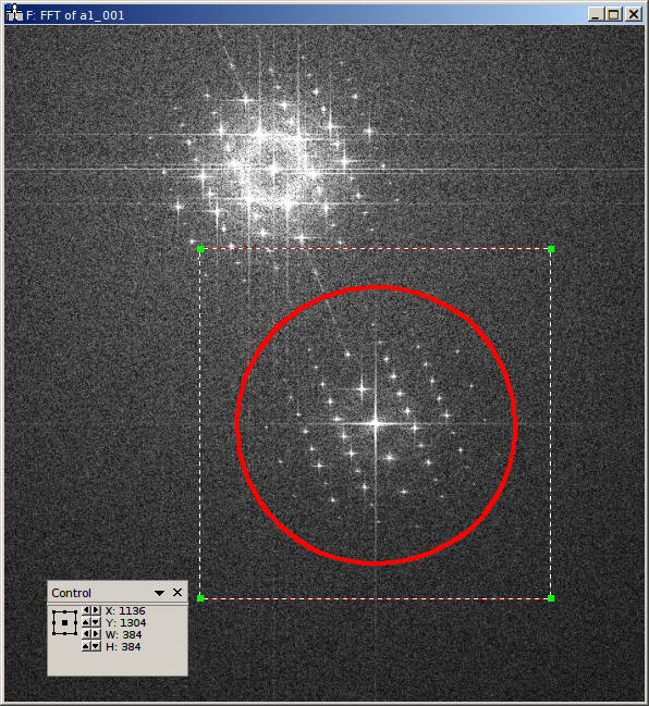
In the figure above, the radius of the red circle is 14.5 1/nm (measured using the Fourier transformed image, after recalibration; see sampling parameter above). This radius in reciprocal nanometers is given by the cut_off parameter. Here, we use an aperture with a soft edge, which is specified by providing the string "BUTTERWORTH" and the order of the Butterworth function (here 14) as filter_func parameter. For a hard edge, simply provide the string "EDGE" instead of the squared parenthesis.

"cut_off" : 14.5,
"filter_func" : ["BUTTERWORTH", 14],

Due to this masking in Fourier space, the reconstructed holograms will have a lower resolution than the original holograms. Thus the resulting data arrays can made smaller, which also speeds up the averaging process. It is sufficient to make the result arrays only as large, that the mask defined above is fully contained within them. As we use a soft edge we give here a little leeway and make the result array 384 pixels large (for performance reasons you should prefer sizes with small prime factors here):

"object_size" : 384,

Another parameter needed for the reconstruction is the region of the object holograms, which should be reconstructed. If the specimen is drifting strongly, not the whole region of the holograms might be present in all acquisitions of the series. In this cases it might be meaningful to only reconstruct a sub region of the hologram:

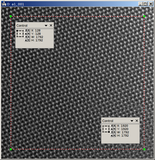
This region is provided to the image program as roi parameter. This region of interest (ROI) is defined as rectangular area in the first object hologram. During the raw-alignment step of the reconstruction, this region is tracked and the same sub-region is extracted from the consecutive object holograms. The left, top, bottom, and right borders are provided to the program in pixel coordinates. As shown in the above figure, the “Control” panel can be used to determine these coordinates, by clicking on the respective corners of the rectangle in the panel. Here only the central 7/8 of the holograms are used, the coordinates are given as left (128), top (128), right (1920), and bottom (1920):

"roi" : [128, 128, 1920, 1920],

If this parameter is omitted, the whole hologram area is used for reconstruction. Please note, that also the region used for raw alignment can be specified explicitly using the align_roi parameter. Alternatively, the raw alignment can be disabled by setting the enable_raw_alignment parameter to false.

The empty hologram series is always reconstructed using the full image region. This is done, for two reasons. For one, there is no specimen drift in empty holograms. For another, the reconstructed empty hologram is used to remove some distortions of the camera and the projection system of the microscope. This are fixed to the camera pixels. The normalization of the object holograms is made with the corresponding sub-region (tracked for specimen drift) of the reconstructed empty hologram. This requires the empty hologram reconstruction to cover the whole camera area.

The reconstruction size of the empty holograms can be chosen independently, and is made a little bit larger here:

"empty_size" : 512,

If the whole hologram area is reconstructed in the object series, the empty_size parameter should be chosen identically to the object_size parameter.

Output and averaging

One has to select which drifts are tracked in the averaging step. By default only specimen drift is tracked and adjusted. Here we also want to track and adjust for focal variations. These adjustments are selected by the following parameters.

"adjust_defocus" : true,
"adjust_shift" : true

When the interference pattern is smaller than the area of the hologram, the amplitude normalization of the flat-field correction might produce strong artifacts. In these cases, it might be beneficial to only normalize the phases of the reconstructions. This can be adjusted by the only_phase parameter. You should also consider to use the align_roi parameter in cases of smaller interference patterns.

"only_phase": false,

Eventually, the filename of the output file must be provided by the output_name parameter. The output will be always HDF5 files, the contents of these files is described in Section Outputs.

"output" : "a1.hdf5",

Starting the program

When correctly installed, the program should be executable from the console. Change into the directory, where your tutorial data files are located, using the cd command of the console. Below it is assumed this directory is called directory-with-data-files, so adjust the path directory-with-data-files below accordingly. Note, you may have to enter the absolute path to the directory. Windows user might also have to switch the current drive they are working with; for that use the desired drive letter, followed by a colon as command (e.g. D:, if the data is located on drive D:) before using the cd command.

cd directory-with-data-files

Now call the holoaverage program and pass the name of the parameter file holoaverage-a1.json to it as argument. The switch -v is optional and enables verbose output.

holoaverage -v holoaverage-a1.json

The program now should start with the reconstruction and averaging and should output something like:

Loading parameters from
        /home/niermann/PycharmProjects/holoaverage/example/holoaverage-a1.json
Loading...
        20 datasets, shape=(2048, 2048), dtype=int16
        [00] GaN_holographic_focal_series/empty_001.dm3
        [01] GaN_holographic_focal_series/empty_002.dm3
        [02] GaN_holographic_focal_series/empty_003.dm3
        [03] GaN_holographic_focal_series/empty_004.dm3
        [04] GaN_holographic_focal_series/empty_005.dm3
        [05] GaN_holographic_focal_series/empty_006.dm3
        [06] GaN_holographic_focal_series/empty_007.dm3
        [07] GaN_holographic_focal_series/empty_008.dm3
        [08] GaN_holographic_focal_series/empty_009.dm3
        [09] GaN_holographic_focal_series/empty_010.dm3
        [10] GaN_holographic_focal_series/empty_011.dm3
        [11] GaN_holographic_focal_series/empty_012.dm3
        [12] GaN_holographic_focal_series/empty_013.dm3
        [13] GaN_holographic_focal_series/empty_014.dm3
        [14] GaN_holographic_focal_series/empty_015.dm3
        [15] GaN_holographic_focal_series/empty_016.dm3
        [16] GaN_holographic_focal_series/empty_017.dm3
        [17] GaN_holographic_focal_series/empty_018.dm3
        [18] GaN_holographic_focal_series/empty_019.dm3
        [19] GaN_holographic_focal_series/empty_020.dm3
Reconstructing...
        . . . . . . . . . . . . . . . . . . . .
Optimizing after iteration 0
        [NN] sx[px] sy[px] tx[1/px] ty[1/px] def[nm] Ampl   Phase  Error
        [00]  0.000  0.000  0.00000  0.00000   0.000 1.0000 +0.802 2.403186e+09
        [01]  0.000  0.000  0.00000  0.00000   0.000 1.0000 -0.672 2.365460e+09
        [02]  0.000  0.000  0.00000  0.00000   0.000 1.0000 -1.478 2.599819e+09
        [03]  0.000  0.000  0.00000  0.00000   0.000 1.0000 -2.849 2.534287e+09
        [04]  0.000  0.000  0.00000  0.00000   0.000 1.0000 -1.102 2.451658e+09
        [05]  0.000  0.000  0.00000  0.00000   0.000 1.0000 +0.163 2.365165e+09
        [06]  0.000  0.000  0.00000  0.00000   0.000 1.0000 +0.439 2.400905e+09
        [07]  0.000  0.000  0.00000  0.00000   0.000 1.0000 -0.745 2.470458e+09
        [08]  0.000  0.000  0.00000  0.00000   0.000 1.0000 +0.303 2.364581e+09
        [09]  0.000  0.000  0.00000  0.00000   0.000 1.0000 +1.830 2.513006e+09
        [10]  0.000  0.000  0.00000  0.00000   0.000 1.0000 +1.208 2.377789e+09
        [11]  0.000  0.000  0.00000  0.00000   0.000 1.0000 -0.781 2.302518e+09
...

and so on. Eventually it should output something like:

Iteration   7: total error=7.501946e+07

This error number should go down and converge to a stable value within the last iterations.

Results

After the program succeeded the outputs can be found in the output file as specified by the output_name parameter. In the present example the outputs are in the file a1.hdf5 in the same directory as the parameter file.

If you are using Digital Micrograph, there is also a plugin to read HDF5 files, which can be found at https://github.com/niermann/gms_plugin_hdf5/releases. These outputs should be checked for artifacts.

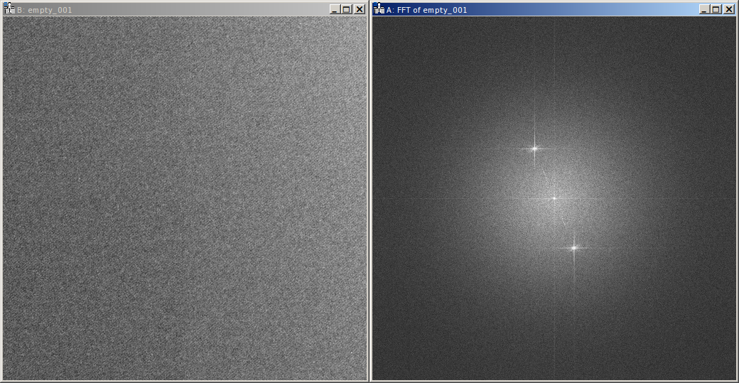
The averaged empty reconstruction is contained in the HDF5 file as dataset empty. It should be more-or-less homogeneous. If the interference only covers the camera partially, only the area of the interference pattern should be homogeneous obviously. Also Fresnel fringes might cause small deviations, the central area of the interference region should be homogeneous nevertheless. Here the phase (left) and amplitude (right) of the empty example series are shown.

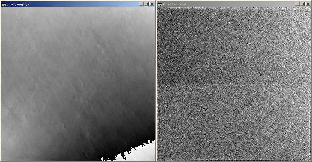
The patterns present in the phase are the aforementioned camera and projection distortions.

The reconstructed object series can be found in the dataset data of the HDF5 file. Here the amplitude (left), phase (center), and Fourier transform (right) of the averaged reconstruction are shown:

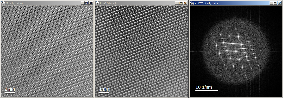
Please note, that this object hologram doesn’t show the GaN structure perfectly, due to residual aberrations. But since you now have reconstructed the full complex information you can now correct for aberrations a-posteriori.

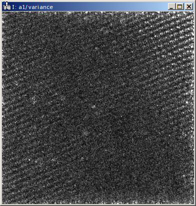
Finally, the variance estimation of the averaging step should be checked. The reconstruction shown above represents the average of the object series. When the object series is averaged, also the variance of the object series (drift corrected and propagated to the Gaussian focus) is checked. This variance for each pixel of the reconstructed object hologram is provided in the dataset variance of the HDF5 file. Small variances (compared to the amplitude values) are to be expected especially at positions with strong contrasts (specimen edges etc.). Also hot pixels of single holograms might pop up in the variance array. However, strong variance indicate a problem with either the data or the averaging process.